Plotting Graphs with `GraphMakie.jl`

The `graphplot` Command

Plotting your first AbstractGraph from Graphs.jl is as simple as

using CairoMakie
using GraphMakie
using Graphs
using StableRNGs

g = wheel_graph(10)
f, ax, p = graphplot(g)
hidedecorations!(ax); hidespines!(ax)
ax.aspect = DataAspect()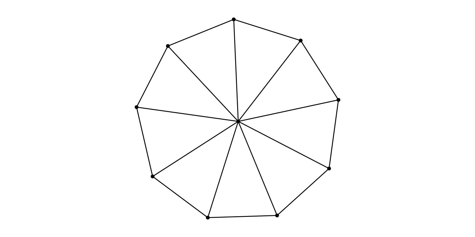

The graphplot command is a recipe which wraps several steps

layout the graph in space using a layout function,
create a scatter plot for the nodes and
create a lines plot for the edges.

The default layout is Spring() from NetworkLayout.jl. The layout attribute can be any function which takes an AbstractGraph and returns a list of Point{dim,Ptype} (see GeometryBasics.jl objects where dim determines the dimensionality of the plot.

Besides that there are some common attributes which are forwarded to the underlying plot commands. See graphplot.

using GraphMakie.NetworkLayout

g = SimpleGraph(5)
add_edge!(g, 1, 2); add_edge!(g, 2, 4);
add_edge!(g, 4, 3); add_edge!(g, 3, 2);
add_edge!(g, 2, 5); add_edge!(g, 5, 4);
add_edge!(g, 4, 1); add_edge!(g, 1, 5);

# define some edge colors
edgecolors = [:black for i in 1:ne(g)]
edgecolors[4] = edgecolors[7] = :red

f, ax, p = graphplot(g, layout=Shell(),
                     node_color=[:black, :red, :red, :red, :black],
                     edge_color=edgecolors)

hidedecorations!(ax); hidespines!(ax)
ax.aspect = DataAspect()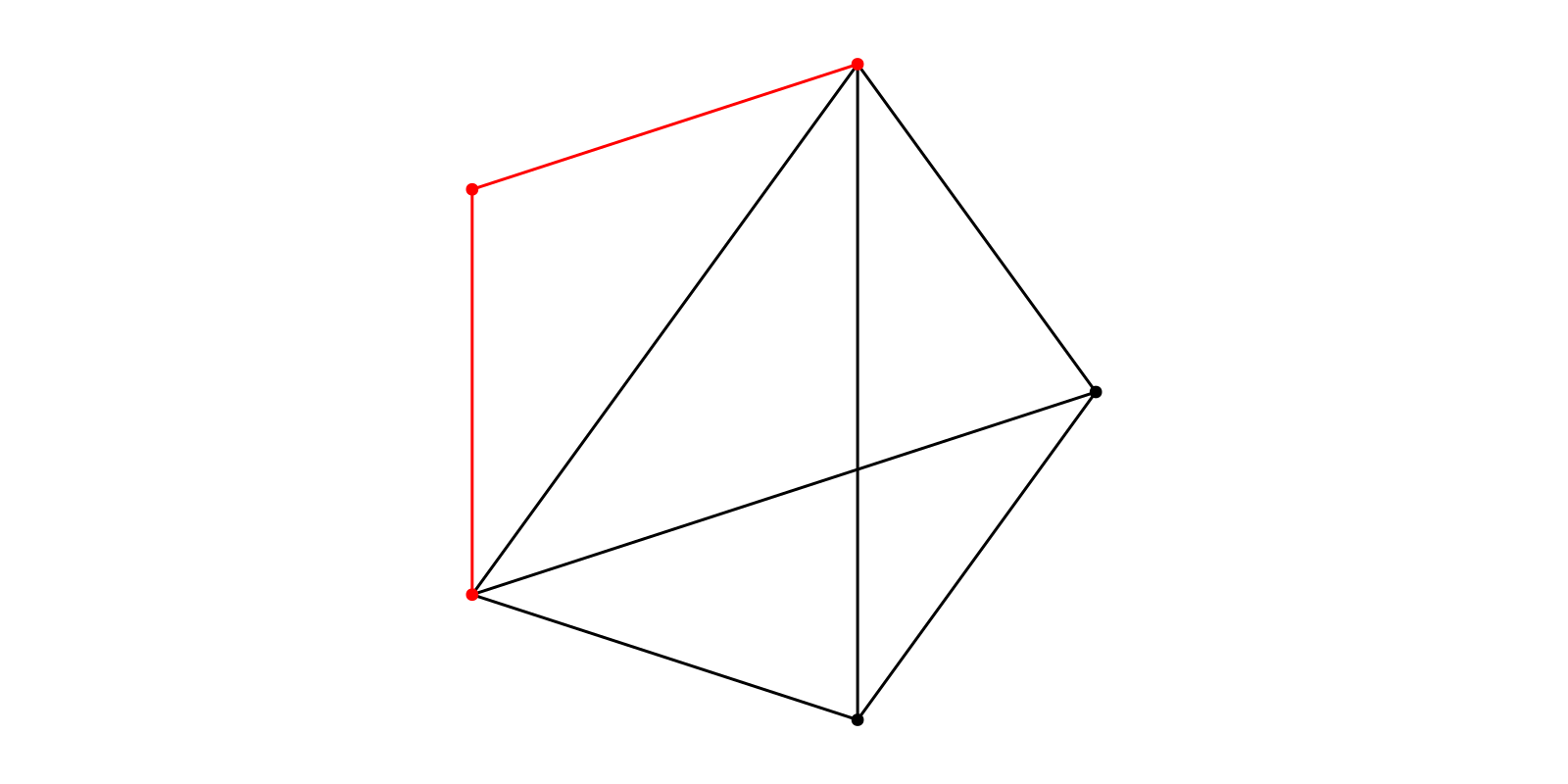

We can interactively change the attributes as usual with Makie.

fixed_layout(_) = [(0,0), (0,1), (0.5, 1.5), (1,1), (1,0)]
# set new layout
p.layout = fixed_layout; autolimits!(ax)
# change edge width & color
p.edge_width = 5.0
p.edge_color[][3] = :green;
p.edge_color[] = p.edge_color[] # trigger observable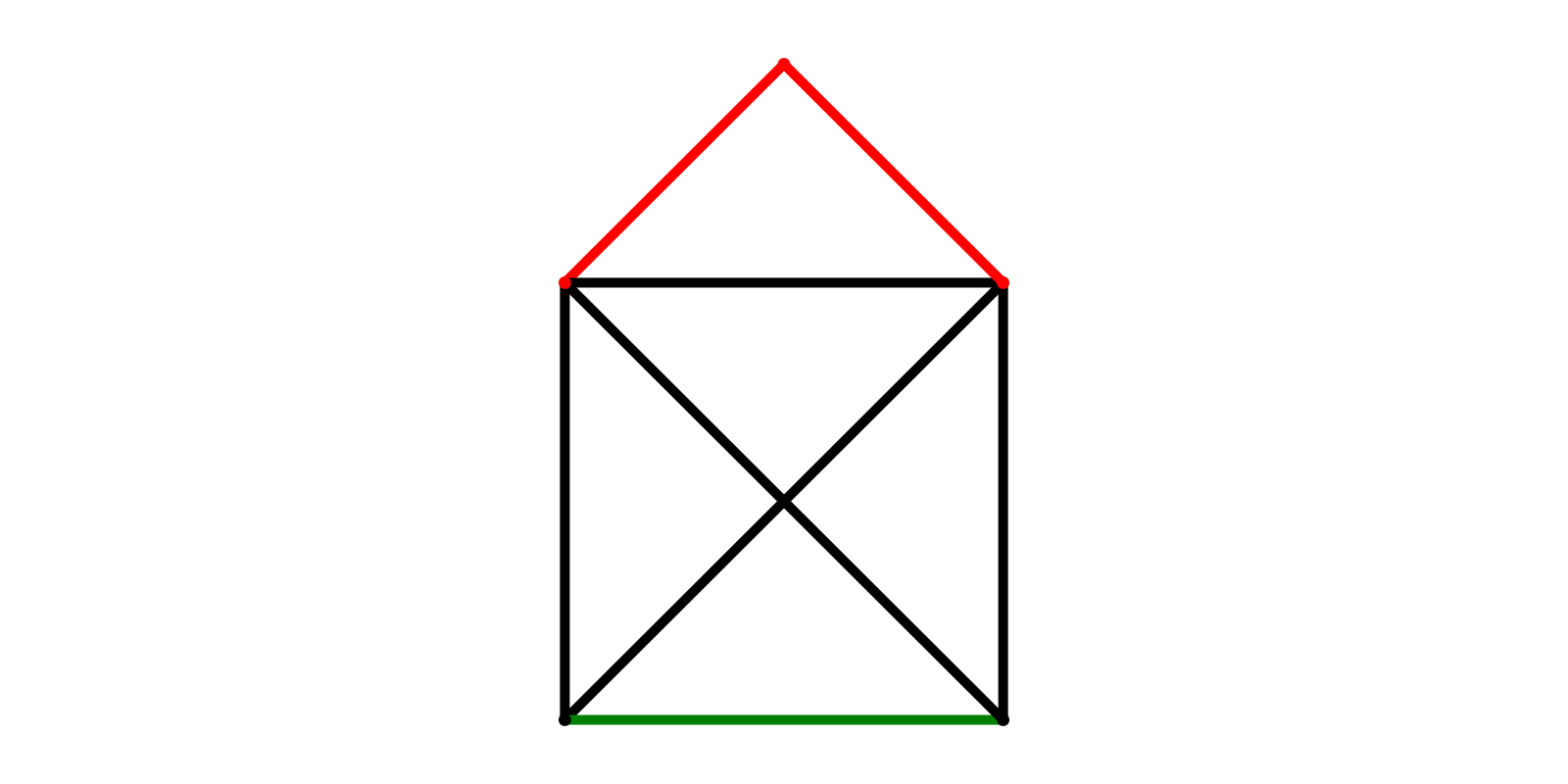

Adding Node Labels

g = wheel_graph(10)

colors = [:black for i in 1:nv(g)]
colors[1] = :red

f, ax, p = graphplot(g,
                     nlabels=repr.(1:nv(g)),
                     nlabels_color=colors,
                     nlabels_align=(:center,:center))
hidedecorations!(ax); hidespines!(ax); ax.aspect = DataAspect()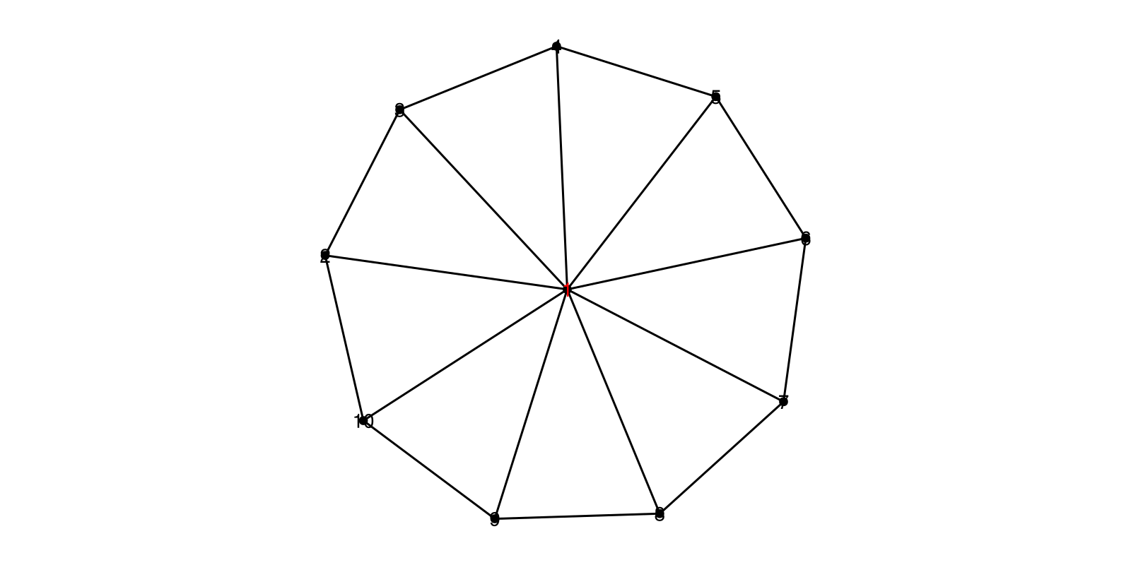

This is not very nice, lets change the offsets based on the node_positions

offsets = 0.15 * (p[:node_pos][] .- p[:node_pos][][1])
offsets[1] = Point2f(0.1, 0.3)
p.nlabels_offset[] = offsets
autolimits!(ax)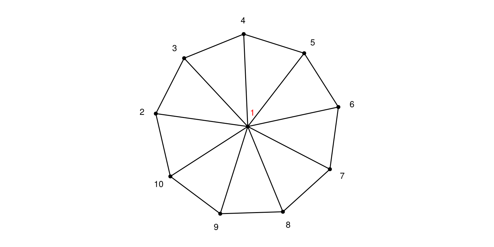

Inner Node Labels

Sometimes it is prefered to show the labels inside the node. For that you can use the ilabels keyword arguments. The Node sizes will be changed according to the size of the labels.

g = cycle_digraph(3)
f, ax, p = graphplot(g;
                     ilabels=[1, L"\sum_{i=1}^n \alpha^i", "a label"],
                     arrow_shift=:end)
xlims!(ax, (-1.5, 1.3))
ylims!(ax, (-2.3, 0.7))
hidedecorations!(ax); hidespines!(ax); ax.aspect = DataAspect()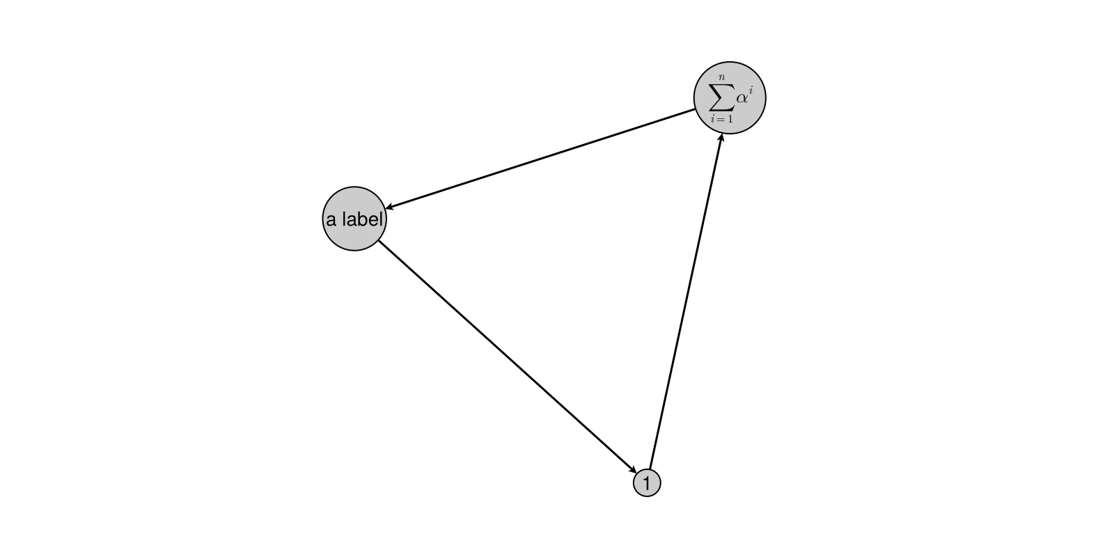

Adding Edge Labels

g = barabasi_albert(6, 2; rng=StableRNGs.StableRNG(1))

labels =  repr.(1:ne(g))

f, ax, p = graphplot(g, elabels=labels,
                     elabels_color=[:black for i in 1:ne(g)],
                     edge_color=[:black for i in 1:ne(g)])
hidedecorations!(ax); hidespines!(ax); ax.aspect = DataAspect()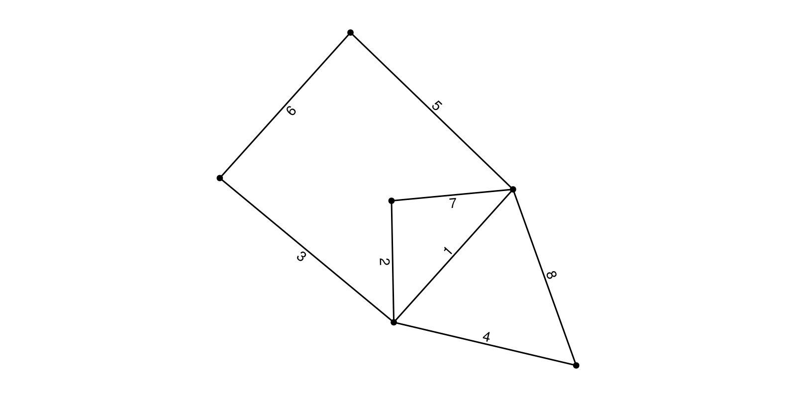

The position of the edge labels is determined by several plot arguments. All possible arguments are described in the docs of the graphplot function.

By default, each label is placed in the middle of the edge and rotated to match the edge rotation. The rotation for each label can be overwritten with the elabels_rotation argument.

p.elabels_rotation[] = Dict(i => i == 2 ? 0.0 : Makie.automatic for i in 1:ne(g))

One can shift the label along the edge with the elabels_shift argument and determine the distance in pixels using the elabels_distance argument.

p.elabels_side[] = Dict(i => :right for i in [6,7])
p.elabels_offset[] = [Point2f(0.0, 0.0) for i in 1:ne(g)]
p.elabels_offset[][5] = Point2f(-0.4,0)
p.elabels_offset[] = p.elabels_offset[]

p.elabels_shift[] = [0.5 for i in 1:ne(g)]
p.elabels_shift[][1] = 0.6
p.elabels_shift[][7] = 0.4
p.elabels_shift[] = p.elabels_shift[]

p.elabels_distance[] = Dict(8 => 30)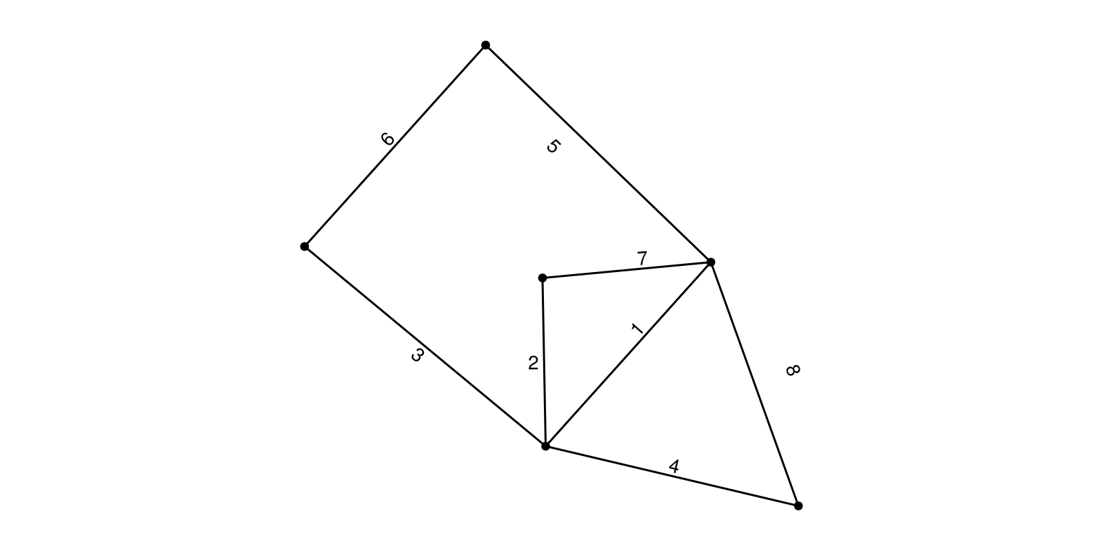

Indicate Edge Direction

It is possible to put arrows on the edges using the arrow_show parameter. This parameter is true for SimpleDiGraph by default. The position and size of each arrowhead can be change using the arrow_shift and arrow_size parameters.

g = wheel_digraph(10)
arrow_size = [10+i for i in 1:ne(g)]
arrow_shift = range(0.1, 0.8, length=ne(g))
f, ax, p = graphplot(g; arrow_size, arrow_shift)
hidedecorations!(ax); hidespines!(ax); ax.aspect = DataAspect()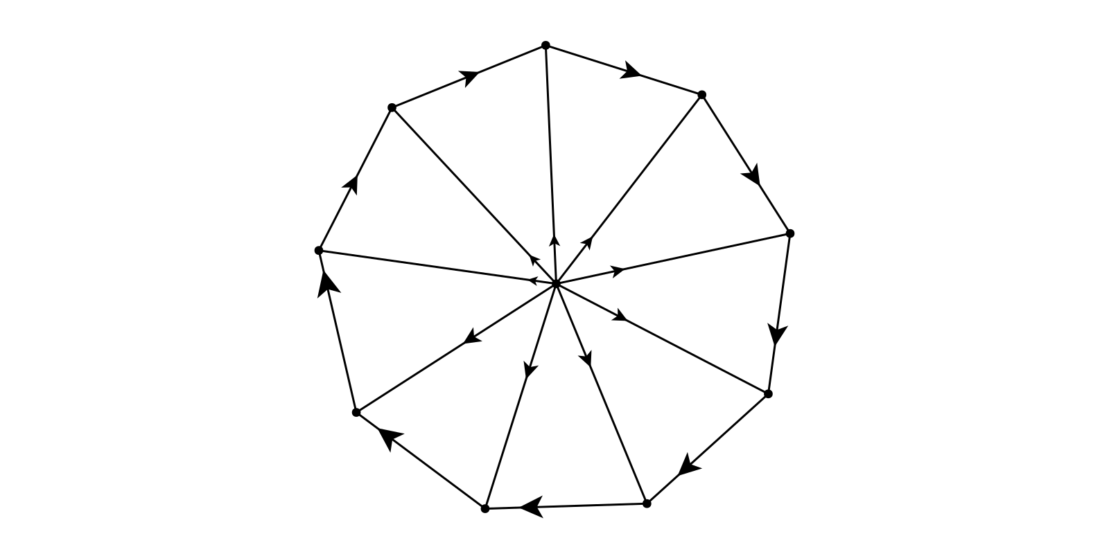

There is a special case for arrow_shift=:end which moves the arrows close to the next node:

g = cycle_digraph(3)
f, ax, p = graphplot(g; arrow_shift=:end, node_size=20, arrow_size=20)
hidedecorations!(ax); hidespines!(ax); ax.aspect = DataAspect()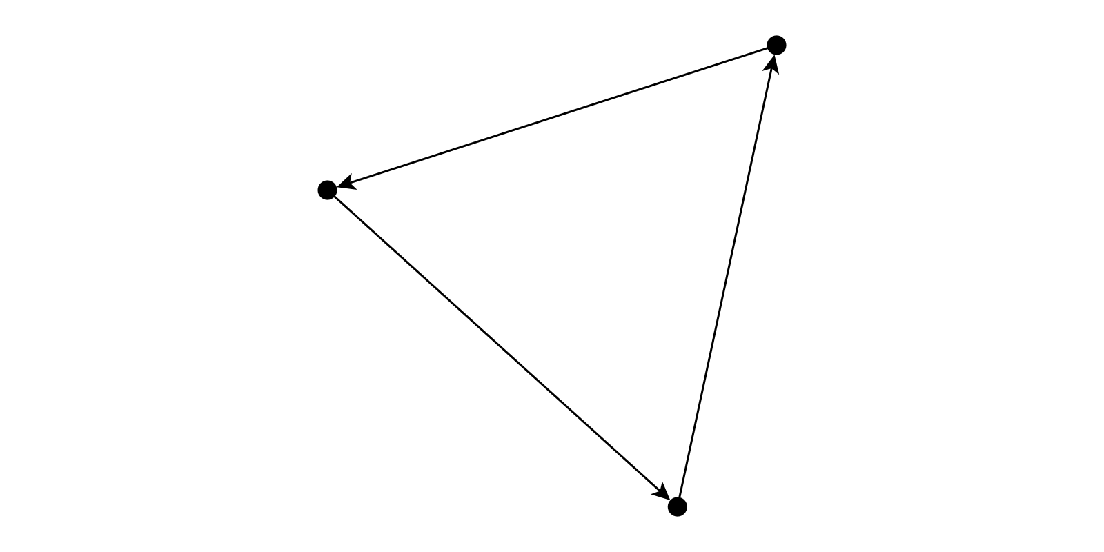

Self edges

A self edge in a graph will be displayed as a loop.

Note

Selfe edges are not possible in 3D plots yet.

g = complete_graph(3)
add_edge!(g, 1, 1)
add_edge!(g, 2, 2)
add_edge!(g, 3, 3)
f, ax, p = graphplot(g)

hidedecorations!(ax); hidespines!(ax); ax.aspect = DataAspect()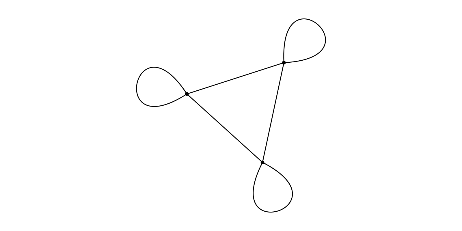

It is possible to change the appearance using the selfedge_ attributes:

p.selfedge_size = Dict(1=>Makie.automatic, 4=>3.6, 6=>0.5) #idx as in edges(g)
p.selfedge_direction = Point2f(-0.25, -0.3)
p.selfedge_width = Any[Makie.automatic for i in 1:ne(g)]
p.selfedge_width[][4] = 0.6*π; notify(p.selfedge_width)
autolimits!(ax)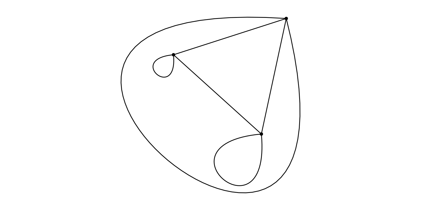

Curvy edges

`curve_distance` interface

The easiest way to enable curvy edges is to use the curve_distance parameter which lets you add a "distance" parameter. The parameter changes the maximum distance of the bent line to a straight line. Per default, only two way edges will be drawn as a curve:

g = SimpleDiGraph(3); add_edge!(g, 1, 2); add_edge!(g, 2, 3); add_edge!(g, 3, 1); add_edge!(g, 1, 3)

f, ax, p = graphplot(g)
hidedecorations!(ax); hidespines!(ax); ax.aspect = DataAspect()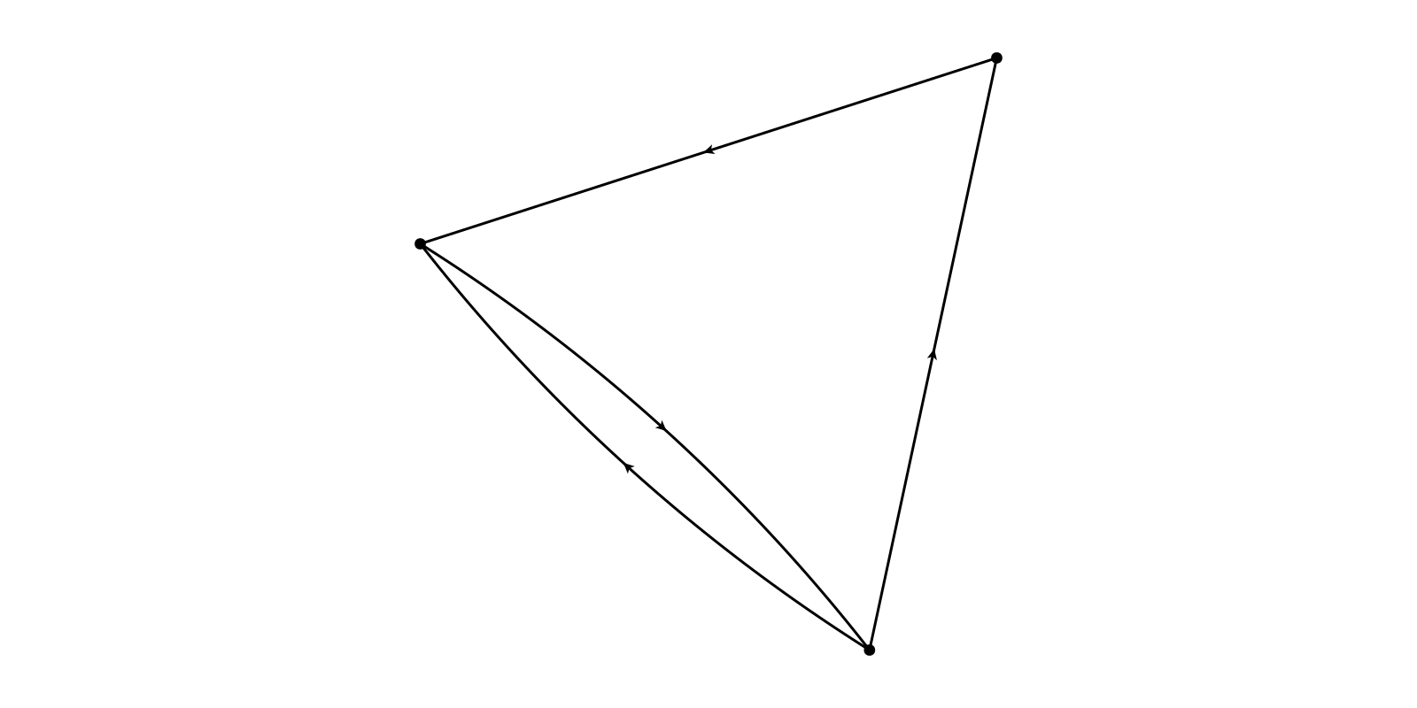

This behaviour may be changed by using the curve_distance_usage=Makie.automatic parameter.

Makie.automatic: Only apply curve_distance to double edges.
true: Use on all edges.
false: Don't use.

f, ax, p = graphplot(g; curve_distance=-.5, curve_distance_usage=true)
hidedecorations!(ax); hidespines!(ax); ax.aspect = DataAspect()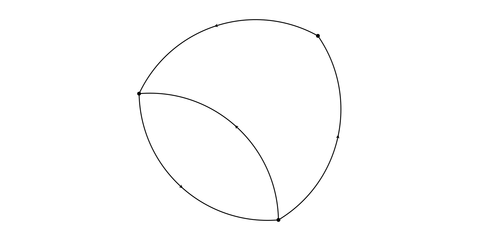

It is also possible to specify the distance on a per edge base:

g = complete_digraph(3)
distances = collect(0.05:0.05:ne(g)*0.05)
elabels = "d = ".* repr.(round.(distances, digits=2))
f, ax, p = graphplot(g; curve_distance=distances, elabels, arrow_size=20, elabels_distance=15)
hidedecorations!(ax); hidespines!(ax); ax.aspect = DataAspect()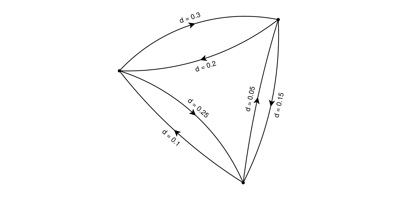

`tangents` interface

Curvy edges are also possible using the low level interface of passing tangent vectors and a tfactor. The tangent vectors can be nothing (straight line) or two vectors per edge (one for src vertex, one for dst vertex). The tfactor scales the distance of the bezier control point relative to the distance of src and dst nodes. For real world usage see the AST of a Julia function example.

using GraphMakie: plot_controlpoints!, SquareGrid
g = complete_graph(3)
tangents = Dict(1 => ((1,1),(0,-1)),
                2 => ((0,1),(0,-1)),
                3 => ((0,-1),(1,0)))
tfactor = [0.5, 0.75, (0.5, 0.25)]
f, ax, p = graphplot(g; layout=SquareGrid(cols=3), tangents, tfactor,
                     arrow_size=20, arrow_show=true, edge_color=[:red, :green, :blue],
                     elabels="Edge ".*repr.(1:ne(g)), elabels_distance=20)
hidedecorations!(ax); hidespines!(ax); ax.aspect = DataAspect()
plot_controlpoints!(ax, p) # show control points for demonstration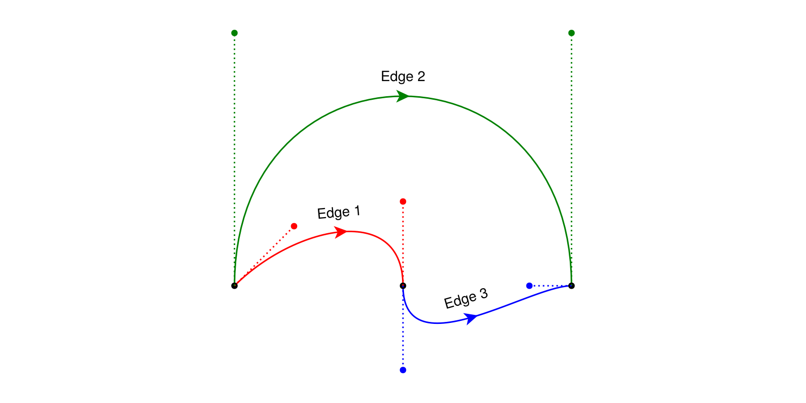

Edge waypoints

It is possible to specify waypoints per edge which needs to be crossed. See the Dependency Graph of a Package example.

If the attribute waypoint_radius is nothing or :spline the waypoints will be crossed using natural cubic spline interpolation. If the supply a radius the waypoints won't be reached, instead they will be connected with straight lines which bend in the given radius around the waypoints.

g = SimpleGraph(8); add_edge!(g, 1, 2); add_edge!(g, 3, 4); add_edge!(g, 5, 6); add_edge!(g, 7, 8)

waypoints = Dict(1 => [(.25,  0.25), (.75, -0.25)],
                 2 => [(.25, -0.25), (.75, -0.75)],
                 3 => [(.25, -0.75), (.75, -1.25)],
                 4 => [(.25, -1.25), (.75, -1.75)])
waypoint_radius = Dict(1 => nothing,
                       2 => 0,
                       3 => 0.05,
                       4 => 0.15)

f = Figure(); f[1,1] = ax = Axis(f)

p = graphplot!(ax, g; layout=SquareGrid(cols=2, dy=-0.5),
               waypoints, waypoint_radius,
               nlabels=["","r = nothing (equals :spline)",
                        "","r = 0 (straight lines)",
                        "","r = 0.05 (in data space)",
                        "","r = 0.1"],
               nlabels_distance=30, nlabels_align=(:left,:center))

xlims!(ax, (-0.1, 2.25)), hidedecorations!(ax); hidespines!(ax); ax.aspect = DataAspect()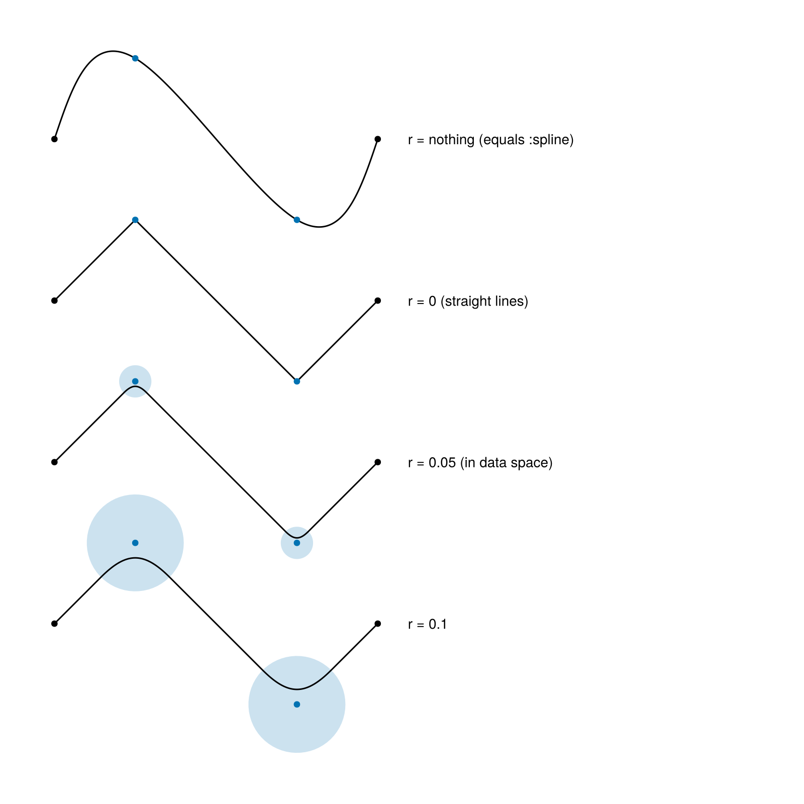

Specifying waypoints for self-edges will override any selfedge_ attributes. If waypoints are specified on an edge, tangents can also be added. However, if tangents are given, but no waypoints, the tangents are ignored.

g = SimpleDiGraph(1) #single node
add_edge!(g, 1, 1) #add self loop
f, ax, p = graphplot(g,
                     layout = [(0,0)],
                     waypoints = [[(1,-1),(1,1),(-1,1),(-1,-1)]])
hidedecorations!(ax); hidespines!(ax); ax.aspect = DataAspect()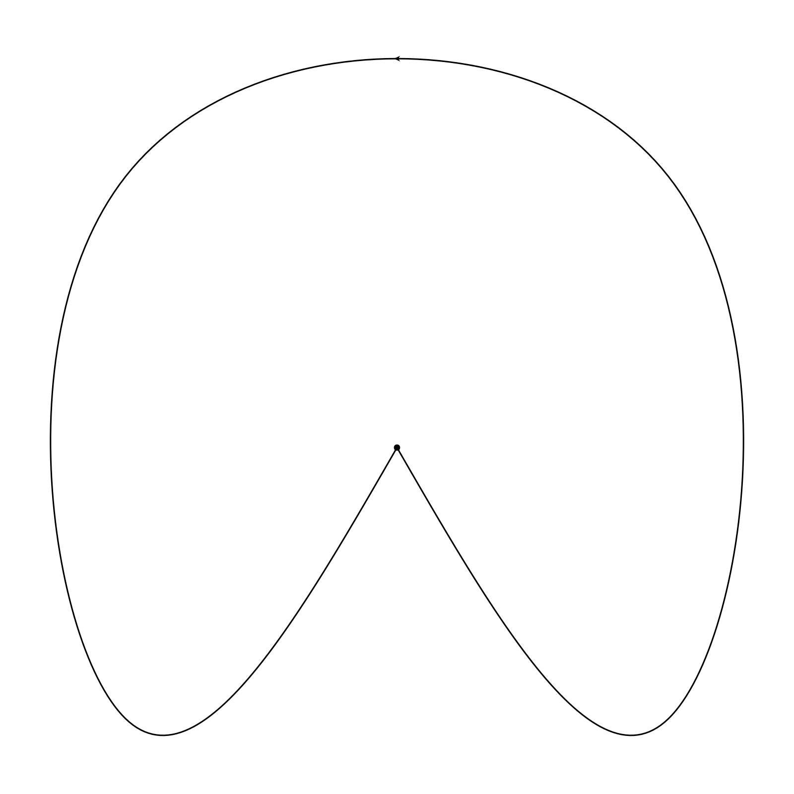

Plot Graphs in 3D

If the layout returns points in 3 dimensions, the plot will be in 3D. However this is a bit experimental. Feel free to file an issue if there are any problems.

g = smallgraph(:cubical)
f, ax, p = graphplot(g; layout=Spring(dim=3, seed=5),
    elabels="Edge ".*repr.(1:ne(g)),
    arrow_show=true,
    arrow_shift=0.9,
    arrow_size=15)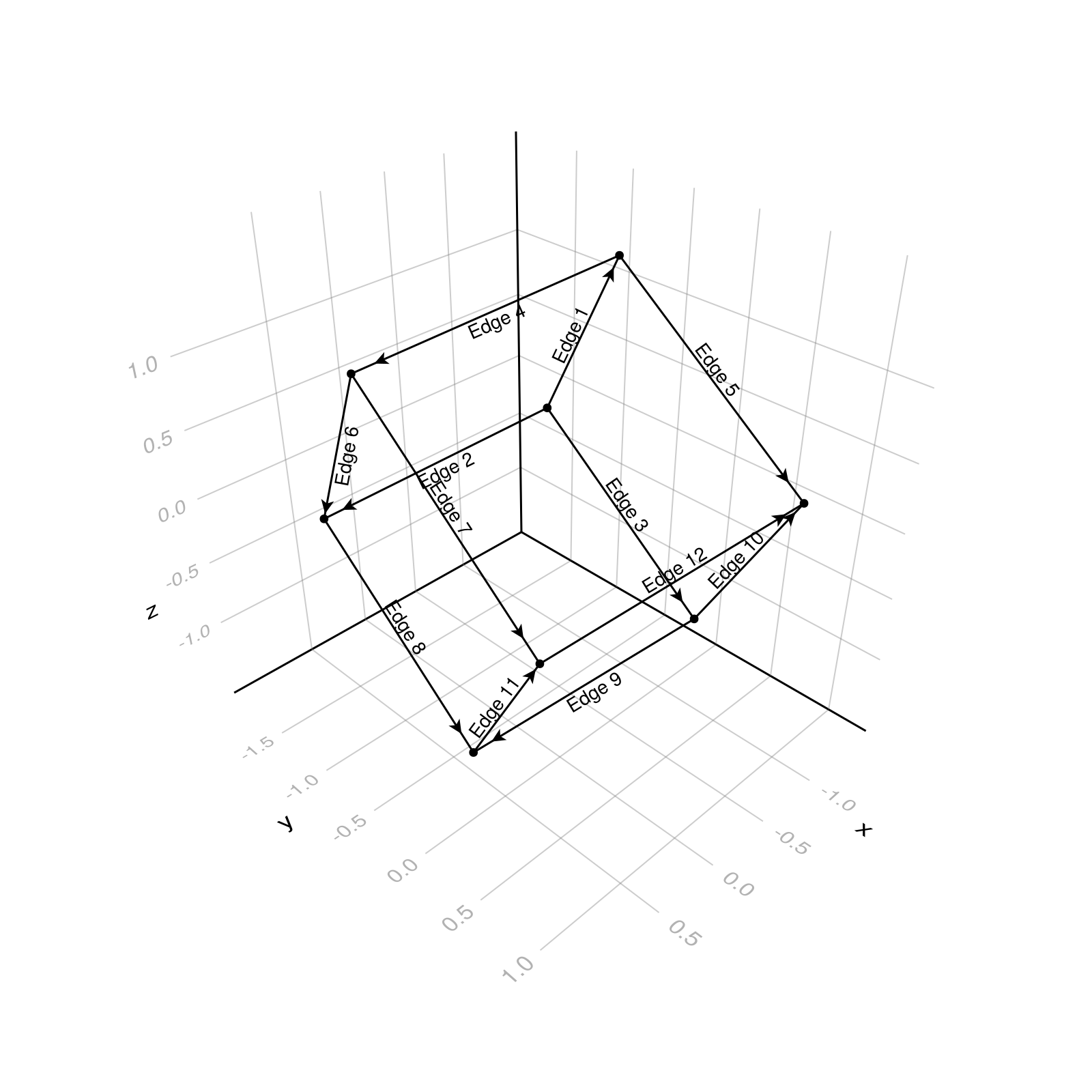

Using WGLMakie.jl we can also add some interactivity:

using WGLMakie
WGLMakie.Page(exportable=true, offline=true)
WGLMakie.activate!()
set_theme!(size=(800, 600))
g = smallgraph(:dodecahedral)
graphplot(g, layout=Spring(dim=3))

This page was generated using Literate.jl.